In this blog post, we explain how our work in learning perturbation sets can bridge the gap between $\ell_p$ adversarial defenses and adversarial robustness to real-world transformations. You can find more details in

Our paper on arXiv here: [Wong & Kolter, 2020]
Our code repository here: [Github]

Introduction
- Overview of adversarial attacks and defenses
Defining perturbation sets with generative modeling
- Necessary subset property
- Sufficient likelihood property
Learning perturbation sets with conditional variational autoencoders
Robustness to learned perturbation sets
Summary

Introduction

Robust deep learning has come a long way from the initial imperceptible adversarial example, having developed a broad range of realistic adversaries such as image transformations, clothing and eyeglasses, and background noise. At the same time, adversarial defenses have also seen advancements, both for empirical defenses (using early stopping and semi-supervised data augmentation) as well as certified defenses (using more scalable bounds and smoothing with optimal noise distributions).

However, there is a significant disparity between real-world attacks and effective adversarial defenses: although adversarial attacks have become increasingly more sophisticated and better reflect real-world transformations, adversarial defenses have largely struggled to expand beyond mathematically “nice” sets like $\ell_p$ balls or other distance metrics. This is largely due to the fact that methods for learning and evaluating adversarially robust models rely heavily on having a well-defined perturbation set (or threat model) which characterizes the set of all possible attacks. Unfortunately, this requirement is fundamentally incompatiable with many real-world attacks, where it may be impossible to mathematically define a perturbation set in the first place. This motivates the fundamental question that we study in this work:

How can we learn models that are robust to perturbations without an a priori specification?

To solve this problem, we propose a simple approach of learning a characterization of the perturbation set from data. At a high level, we learn a conditional generative model that maps a datapoint $x$ and an $\ell_p$ ball in the latent space to real-world perturbations of $x$, resulting in a learned perturbation set. This allows us to get the best of both worlds: we can use state-of-the-art approaches in adversarial defenses in the latent space to learn models which are robust to real-world perturbations captured by the generator.

Overview of adversarial attacks and defenses

We start with a brief description of the typical formulation for adversarial attacks and defenses, and their corresponding strengths and limitations.

Adversarial attacks

Adversarial attacks are typically framed as an optimization problem, where the “adversary” attempts to maximize a loss of a classifier over a set of allowable perturbations. Specifically, for an example $x$ with label $y$, a classifier $h$, and a loss $\ell$, let $\mathcal S(x)$ represent the set of allowable perturbations of $x$. Then, an adversarial example is the solution to

$\underset{x' \in \mathcal S(x)}{\operatorname{argmax}} \ell(h(x'), y)$

Different types of adversarial examples can be obtained by defining or restricting $\mathcal S(x)$. For example, we can define such as set with a generic distance metric $d$ as follows:

$\mathcal S(x) = \{ x' : d(x,x') \leq \epsilon\}$

By taking $d(x,x’) = \|x-x’\|_p$, we get a classic adversarial example meant to capture “imperceptible” unstructured noise also known as the $\ell_p$ adversarial example, where $p$ is commonly taken to be from $\{1, 2, \infty\}$. By using other, more structured metrics, we can get other types of adversarial examples such as the Wasserstein adversarial example from the Wasserstein metric. For images, the distance can arise from well-defined spatial transformations, such as the number of degrees in a rotation or the number of pixels in a translation. However, for many real-world adversarial attacks, $\mathcal S(x)$ may be significantly more complex, and is not so easily defined. For example, realistic transformations that capture changes in lighting, weather effects, or viewing angles may not be so admissable to an exact, mathematical formulation.

For these real-world transformations, the $\ell_p$ perturbation set is quite simply not the right fit. An $\ell_p$ ball with too small a radius will often not contain all of the desired perturbations, and expanding the radius to contain all possible perturbations often results in an unreasonably large perturbation set. Consequently, existing work in realistic adversarial attacks either simply do not constrain the adversary or rely on additional human input to select “reasonable” adversarial examples. These approaches can successfully fool deep learning classifiers, but at the cost of leaving behind the notion of a well-defined perturbation set.

Adversarial defenses

Complementary to adversarial examples are adversarial defenses, which are methods for learning classifiers which are robust to adversarial attacks. Specifically, if $\theta$ parameterizes the classifier $h_\theta$, adversarial defenses can be framed as solving the following min-max optimization problem

$\underset{\theta}{\operatorname{minimize}} \sum_i \underset{x_i' \in \mathcal S(x_i)}{\operatorname{max}} \ell(h_\theta(x_i'), y_i)$

where the goal is to minimize the adversarial empirical loss, as opposed to the standard empirical loss. Adversarial defenses have seen much attention in the setting where $\mathcal S(x)$ is an $\ell_p$ ball, resulting in strong empirical defenses such as adversarial training, as well as provable defenses which minimize a guaranteed upper bound on the adversarial loss. Crucially, all of these approaches rely on the fact that $\mathcal S(x)$ is well-defined in order to directly optimize or bound the inner maximization over $\mathcal S(x)$. Consequently, these defenses have largely focused on the simple $\ell_p$ setting, with little to no existing work on principled defenses against more realistic adversarial transformations.

In this work, we will define a perturbation set over the latent space of a generative model, allowing us to model real-world perturbations while being able to leverage $\ell_p$ adversarial defenses, thus bridging the gap between real-world attacks and $\ell_p$ adversarial defenses.

Defining perturbation sets with generative modeling

The crux of our approach is to define a perturbation set with a conditional generative model, which maps a well-defined perturbation set in the latent space to realistic perturbations. Specifically, suppose we have pairs of examples $(x, \tilde x) \in \mathcal X$, where $\tilde x$ is a perturbed version of $x$. Then, let $g : \mathcal Z \times \mathcal X \rightarrow \mathcal X$ be a conditional generator that maps a latent code $z \in \mathcal Z$ and an example $x$ to a perturbation $\tilde x$. In other words, $g$ perturbs $x$ into $\tilde x$ via a latent code $z$. Then, we can define a learned perturbation set as

$\mathcal S(x) = \{ g(z,x) : \|z\| \leq \epsilon\}$

where changes in $z$ correspond to different perturbations. This characterization of a perturbation set is simple yet quite powerful. By using a deep generative model $g$, this perturbation set is quite flexible and can more accurately capture realistic sets that are significantly more complex than $\ell_p$ balls by training on the perturbed examples $(x, \tilde x)$. At the same time, the perturbation set is well-defined over an $\ell_p$ ball in the latent space, making it well-suited for adversarial robustness settings.

In additional, we can also define a probabilistic version of a perturbation set. By taking a probabilistic graphical modeling perspective, we can use a distribution over the latent space to parameterize a distribution over examples. Specifically, $\mathcal S(x)$ is a random variable defined by

$\mathcal S(x) \sim p_\theta, \quad \theta = g(z,x) , \quad z \sim p_\epsilon$

where $p_\epsilon$ has support $\{z : \|z\| \leq \epsilon\}$ and $p_\theta$ is a distribution parameterized by $\theta = g(z,x)$. This characterization of a perturbation set results in a well-defined generative process that allows us to draw random samples, making it well-suited for average-case robustness.

One should be (rightfully!) suspicious of a perturbation set defined by a deep generative model over a latent space that is learned from data. After all, how do we know whether this perturbation set actually contains real perturbations? What if this perturbation set contains unrealistic perturbations? Since the generator defining the perturbation set is learned from data, we must carefully evaluate the quality of this perturbation set, in order to properly motivate its usage in downstream robustness tasks. In the remainder of this section, we’ll briefly discuss two meaningful criteria that we would like a learned perturbation set to have for robustness settings.

Necessary subset property

One natural criteria that we desire out of our learned perturbation set is that the perturbation set should at least contain close approximations of the perturbed data that we observe, which we call the necessary subset property. More formally, for a perturbed datapoint $(x, \tilde x)$ we say that a perturbation set $\mathcal S(x)$ satisfies the necessary subset property at approximation error $\delta$ if there exists an $x’ \in \mathcal S(x)$ such that $\|x’ - \tilde x\|_2 \leq \delta$.

In other words, this property captures the notion that observations of perturbed data should be, in some sense, a lower bound on the learned perturbation set. By ensuring that the perturbed data is contained within the learned perturbation set, the perturbation set becomes well-motivated for adversarial robustness: the worst-case loss within the learned perturbation set will be an upper bound on the worst-case loss over observations of perturbed datapoints. Note that perturbation sets like the $\ell_p$ ball naturally have zero approximation error (observed $\ell_p$ perturbations are captured exactly by the mathematical characterization).

Sufficient likelihood property

Although the necessary subset property is a good start, it is not quite enough on its own to fully characterize a reasonable perturbation set. For example, if we take a perturbation set to be the entire space of possible outputs $\mathcal S(x) = \mathcal X$, then this perturbation set trivially satisfies the necessary subset property for any observations at zero approximation error. However, this is clearly an unreasonable perturbation set (since it contains everything), and so we need to also limit the scope of a learned perturbation set.

This brings us to our second criterion for perturbation sets that we call the sufficient likelihood property, which says that a perturbation set should output realistic data in expectation. More formally, for a perturbed datapoint $(x, \tilde x)$, we say that a probabilistic perturbation set $\mathcal S(x)$ satisfies the sufficient likelihood property at likelihood at least $\delta$ if $\mathbb E_{p_\epsilon}(z)[p_\theta(\tilde x)] \geq \delta$ where $\theta = g(z,x)$.

In other words, this property captures the notion that a perturbation set should not contain “too much”, since it must assign high likelihood to real data in expectation. This effectively limits the scope of a perturbation set, and motivates its usage as a form of random data augmentation via sampling from the latent space.

In total, these two criteria (the necessary subset and sufficient likelihood properties) capture opposing limits in the form of a lower and upper bound that encourages the perturbation set to reflect real perturbed data.

Learning perturbation sets with conditional variational autoencoders

In this section, we will discuss more concretely how to learn the generator of a perturbation set in practice. In particular, we will use a conditional variational autoencoder to learn the generator, which is a principled way of learning a perturbation set that satisfies the necessary subset and sufficient likelihood properties.

The primary running example we will use is this frog from the CIFAR10 dataset with common corruptions.

plt.imshow(X[0].permute(1,2,0).numpy())
plt.axis('off');

In this example, $x$ is the original CIFAR10 frog, and $\tilde x$ is the same frog but corrupted with one of the following common corruptions (which are roughly grouped into three main categories):

Blurs (defocus, glass, motion, zoom)
Weather (snow, frost, fog)
Digital (brightness, contrast, elastic, pixelate, jpeg)

Although these are synthetically generated by nature, these types of perturbations are not easy to define mathematically and represent a diverse set of transfromations that is not easily captured by $\ell_p$ balls as shown below.

fig = plt.figure(figsize=(6,8))#, linewidth=4, edgecolor="#04253a")
grid = ImageGrid(fig, 111,  # similar to subplot(111)
                 nrows_ncols=(3, 4),  # creates 2x2 grid of axes
                 axes_pad=0.02,  # pad between axes in inch.
                 )
ims = make_grid(grid,hX)

Conditional variational autoencoders

In theory, we could potentially use any generative modeling framework, and train it to output $\tilde x$ conditioned on $x$. However, depending on the generative framework, we are not necessarily guaranteed that the resulting perturbation set satisfies the necessary subset and sufficient likelihood properties described before.

In this work, we specifically use the conditional variational autoencoder (CVAE) framework to learn the generative mapping $g$. The reason for this choice is that the CVAE is a principled way of satisfying the necessary subset and sufficient likelihood properties, which will be shown later. For now, we can train the generator in the standard way for CVAEs, by optimizing the typical log likelihood lower bound as shown in the following code block.

cvae = init_cvae()
opt = optim.Adam(cvae.parameters(), lr=0.001)
for i in range(300): 
    output = cvae(X, hX)
    loss = vae_loss(output)
    if i % 20 == 0: 
        print(loss.item())
    
    opt.zero_grad()
    loss.backward()
    opt.step()

113.59719848632812
40.59444808959961
29.130046844482422
19.32047462463379
15.265201568603516
14.203840255737305
12.135712623596191
11.395207405090332
11.032021522521973
10.287261962890625
9.996268272399902
9.488751411437988
9.547000885009766
9.293497085571289
8.202948570251465

where we can check the reconstructions and observe that the VAE has indeed learned how to reconstruct the perturbed versions of the frog.

fig = plt.figure(figsize=(6,8))#, linewidth=4, edgecolor="#04253a")
grid = ImageGrid(fig, 111,  # similar to subplot(111)
                 nrows_ncols=(3, 4),  # creates 2x2 grid of axes
                 axes_pad=0.02,  # pad between axes in inch.
                 )
ims = make_grid(grid,output[0])

Although VAEs have historically struggled to generate accurate, non-blurry images, we note that our CVAEs do not suffer from this problem. By conditioning on another example, the CVAE merely needs to learn how to perturb an image, and does not need to learn to reconstruct an entire image. Consequently, the reconstructions and samples of perturbed images from the CVAE are actually rather accurate, in contrast to the typical VAE setting.

From CVAE to perturbation sets

We can now extract the generator from the CVAE to get our perturbation set. Let $\mathcal N(\mu(x), \sigma(x))$ be the prior distribution for the latent space of the CVAE conditioned on $x$. The generative process of a CVAE that generates $\tilde x$ from $z$ conditioned on $x$ can be written as (see the CVAE paper by Sohn et al. 2015 for a more complete description)

$z \sim \mathcal N(0,I), \quad \tilde x \sim \mathcal N(g(\sigma(x)\cdot z + \mu(x),x), I).$

Note that we’ve decided to write $z$ as the latent space before the reparameterization trick, effectively treating the reparameterization trick as part of the generator. So the complete generator for the perturbation set involves three steps: (1) calculating the prior distribution, (2) performing the reparameterization trick, and (3) passing the latent code through the decoder, as shown in the following code block:

def generator(X,z): 
    prior_params = cvae.prior(X)
    z = cvae.reparameterize(prior_params, z)
    return cvae.decode(X,z)

This choice in notation allows us to use a consistent underlying latent space for all examples, a standard Normal distribution with zero mean and unit variance. Then, we can get a perturbation set by restricting the latent space to an $\ell_2$ ball and taking the output of the generator $g$ (the mean of the likelihood)

$\mathcal S(x) = \{g(\sigma(x) \cdot z + \mu(x),x) : \|z\|_2 \leq \epsilon\}$

and we can also get an analogous probabilistic perturbation set by simply truncating the prior distribution for $z$ to a radius $\epsilon$:

$\mathcal S(x) \sim \mathcal N(\theta, I),\quad \theta = g(\sigma(x)\cdot z + \mu(x),x), \quad z \sim \mathcal N_\epsilon(0,I)$

For the rest of this notebook, we will omit the reparameterization trick and put it implicitly within the generator, and so $g(z,x)$ will refer to $g(\sigma(x)\cdot z + \mu(x),x)$.

Selecting a radius

One natural question to ask at this point is how do we choose the radius of the perturbation set $\epsilon$? This parameter directly controls how expressive or restricted the perturbation set is. Higher values of $\epsilon$ will allow for a more freedom in the generated images, allowing the perturbation set to more accurately capture real-world transformations but at the risk of containing extra perturbations that are not necessarily real. On the other hand, a lower value of $\epsilon$ will restrict the perturbation set to not contain extraneous perturbations, but at the risk of not accurately capturing all desired real-world transformations.

Since we care about worst-case robustness, in this notebook we take a computationally efficient yet conservative approach, and ensure that all perturbed datapoints are accurately represented in the perturbation set. Specifically, we select the largest norm of the posterior means for perturbed data, effectively guaranteeing that the perturbation set contains all of the posterior means of the perturbed data. If we let $\mu(x,\tilde x)$ be the mean of the posterior for the CVAE, and let $\mu(x), \sigma(x)$ be the mean and variance of the prior, then $\epsilon$ can be estimated as

$\epsilon = \max_{(x, \tilde x)} \left\|\frac{\mu(x, \tilde x) - \mu(x)}{\sigma(x)}\right\|_2.$

We can demonstrate this calculation in the following code block, where we find all the CVAE reconstructions of the frog lie within a radius of $\epsilon=11$:

(mu_prior, logvar_prior), (mu_recog, logvar_recog) = cvae.encode(X, hX)
std = torch.exp(0.5*logvar_prior)

epsilon = ((mu_recog - mu_prior)/std).norm(p=2,dim=1).max()
print(f"Maximum epsilon: {epsilon.item()}")

Maximum epsilon: 10.576871871948242

Since the posterior mean of a CVAE is trained to reconstruct perturbed data, this estimate ensures that the resulting perturbation set contains reasonably accurate versions of the perturbed data. Although we could potentially refine this $\epsilon$ even further, for our purposes the CVAE posterior provides a reasonably effective and computationally cheap way to estimate the $\epsilon$ radius. To ensure that the radius is not overfitted to the training set, in general one should use hold-out validation set for computing the final $\epsilon$ in order for the perturbation set to properly generalize to unseen data.

Theory of CVAEs and perturbation sets

So why did we use a CVAE in the first place, and why does this result in a reasonable perturbation set? We can now discuss our main theoretical results, which are to show that optimizing the CVAE objective results in perturbation sets that satisfy the necessary subset and sufficient likelihood properties. This is the underlying reason why the CVAE framework is a principled approach for learning real-world perturbation sets, which may not be true of other generative frameworks like GANs.

More concretely, for a perturbed datapoint $(x,\tilde x)$, CVAEs are trained by maximizing a lower bound on the log likelihood (denoted as $\ell_\textrm{CVAE}$):

$\log p(\tilde x | x) \geq \ell_\textrm{CVAE}(\tilde x, x)$

Then, we can show theoretically that for a radius $r$, that if $\ell_\textrm{CVAE}(\tilde x, x) \geq L$, then the perturbation set defined by the generator of this CVAE with radius $\epsilon(L, r)$ satisfies the aforementioned necessary subset property at approximation error at most $\delta(L, r)$. Furthermore, as the CVAE objective approaches its theoretically optimal objective $L \rightarrow L^\star$, then $\epsilon \rightarrow r$ and $\delta \rightarrow 0$. In other words, the CVAE objective results in a bound on the approximation error of the perturbation set, and so training a CVAE naturally results in a perturbation set which satisfies the necesssary subset property.

In practice, we can calculate the approximation error of the perturbation set by solving the following optimization problem, which searches over the latent space for a latent code which best approximates $\tilde x$ as a perturbation of $x$:

$\min_{\|z\| \leq \epsilon} \|g(z,x) - \tilde x\|_2^2$

This can be calculated with projected gradient descent and can be be warm-started with the posterior mean, as shown in the following code block.

def necessary_subset(X, hX, generator, z=None, epsilon=11): 
    if z is None: 
        z = torch.randn(X.size(0),latent_dim)
    opt = optim.Adam([z], lr=0.1)
    for i in range(50): 
        z.requires_grad = True
        approx_err = F.mse_loss(generator(X,z), hX)
        
        opt.zero_grad()
        approx_err.backward()
        opt.step()
        
        with torch.no_grad(): 
            z.data = z.renorm(2, 1, epsilon)
            if i % 10 == 0 or i == 49: 
                print(approx_err.item())
    return z.detach()

# z = necessary_subset(X,hX, generator, z=((mu_recog - mu_prior)/std).detach())
z = necessary_subset(X,hX, generator)

0.01652415283024311
0.0037946028169244528
0.0023903599940240383
0.0019773689564317465
0.0017868711147457361
0.0016655608778819442

Our running example of the CIFAR10 perturbation set for the image of a frog, using the radius $\epsilon=11$ as calculated previously, is able to approximate the original perturbed datapoints at less than $0.002$ mean squared error. By accurately containing the original perturbed datapoints, we can be more confident that worst-case robustness against this set results in worst-case robustness to real data.

Our second main theoretical result is that for a radius $r$, if $\ell_\textrm{CVAE}(\tilde x, x) \geq L$, then the perturbation set defined by the generator of this CVAE with radius $r$ satisfies the sufficiently likelihood property with likelihood at least $\delta(L, r)$. In other words, the CVAE objective results in a lower bound on the expected likelihood of the perturbation set, and so training a CVAE naturally results in a perturbation set which satisfies the sufficient likelihood property.

In practice, we can estimate the sufficient likelihood property by sampling from the truncated prior as shown below (note that computing the MSE is equivalent to computing the likelihood, due to the parameterization of the CVAE with Normal distributions):

def sufficient_likelihood(X, hX, generator, samples=10, epsilon=11): 
    approx_err = 0
    for i in range(samples): 
        z = utilities.torch_truncnorm(epsilon, X.size(0),latent_dim)
        approx_err += F.mse_loss(generator(X,z), hX)
        
    print(approx_err.item()/samples)

# z = necessary_subset(X,hX, generator, z=((mu_recog - mu_prior)/std).detach())
sufficient_likelihood(X,hX, generator)

0.017223326861858367

The perturbation set in this notebook for the frog has an expected approximation error of $0.017$. By bounding the expected approximation error (and consequently the expected likelihood), we can be confident that the perturbation set doesn’t stray too far from real examples, since it must output an approximation of real examples in expectation.

These results provide theoretical and practical justification for why CVAEs are a principle approach for learning perturbation sets. We conclude this section by noting that the proofs for these results are not so straightforward, and require several supporting results. These rely heavily on the multivariate normal parameterizations of the CVAE distributions in order to transfer the log likelihood lower bound using the posterior into a bound on the approximation error of a perturbation set centered around the prior. For more details and to see how we prove this check out our theorems in the paper.

Robustness to learned perturbation sets

The first half of this notebook established how to define, learn, and evaluate a perturbation set trained from examples. We now shift gears towards demonstrating how these perturbation sets can be used in downstream robustness tasks. This turns out to be quite simple: since our perturbation sets are defined over an $\ell_p$ ball in the latent space, existing approaches for $\ell_p$ adversarial robustness can be naturally and directly applied to this perturbation set. Specifically, any robust training or certification procedure that works for norm-bounded perturbations can be applied to the latent space of the generator. Since the multivariate Normal distributions used in CVAEs naturally lends to a perturbation set based on the $\ell_2$ norm, we will focus on adversarial defenses for $\ell_2$ perturbations, namely adversarial training and randomized smoothing.

Adversarial examples for learned perturbation sets

A typical approach for generating $\ell_2$ adversarial examples is to use projected gradient descent to maximize the loss of a classifier. For images, this is commonly done in the pixel space (the input to the classifier) to model $\ell_2$ perturbation sets that capture random additive noise. This can be adapted to our learned perturbation sets in a fairly straightforward manner: simply run projected gradient descent in the latent space of the generator to maximize the loss of the classifier! Mathematically, this amounts to solving the following optimization problem

$\max_{\|z\|\leq \epsilon} \ell(h(g(x,z)), y)$

where $\mathcal S(x) = \{g(x,z) : \|z\| \leq \epsilon\}$ is the learned perturbation set from before, $h$ is the classifier being attacked, and $\ell$ is some loss (e.g. cross entropy loss). This may look very familiar: if we consider the composition of the classifier with the generator, $h \circ g(x, \cdot)$, to be a deep network, then this is identically the same type of optimization problem for generating standard $\ell_p$ adversarial examples. Consequently, we can run a typical $\ell_2$ PGD adversary in the latent space in order to solve this problem and generate adversarial examples, as shown in the following code block:

latent_dim = 128
def pgd(classifier, generator, X, y, epsilon=11, alpha=0.2, niters=7): 
    # zero initialization for simplicity, but can use random initialization
    batch_size = X.size(0)
    z = X.new_zeros(batch_size, latent_dim)
    
    for i in range(niters):
        with torch.enable_grad():
            z.requires_grad = True

            # generate perturbed image
            X_adv = generator(X, z)
            output = classifier(X_adv)

            # compute loss and backward
            loss = F.cross_entropy(output, y)
            loss.backward()

        with torch.no_grad(): 
            # take L2 gradient step
            g = z.grad
            g = g / g.norm(p=2,dim=1).unsqueeze(1)
            z = z + alpha * g
            # project onto ball of radius max_dist
            z = z.renorm(2,1,epsilon)
        z = z.clone().detach()
    
    return generator(X,z)

This allows us to easily generate adversarial examples within the learned perturbation set. For example, for the CIFAR10 image of a frog, we can generate an adversarial example for a typical CIFAR10 classifier that misclassifies the attacked image as a cat as seen below. The resulting corrupted example turns out to be a blurring corruption, one of many corruptions that the CVAE was trained to produce. The key point here is that we were able to learn a semantically meaningful perturbation set using a CVAE, and so adversarial examples generated in this perturbation set also result in semantically meaningful perturbations which cannot be directly expressed as a set of mathematical constraints.

X_adv = pgd(classifier, generator, X, y)

fig = plt.figure(figsize=(6,8))#, linewidth=4, edgecolor="#04253a")
grid = ImageGrid(fig, 111,  # similar to subplot(111)
                 nrows_ncols=(1, 2),  # creates 2x2 grid of axes
                 axes_pad=0.2,  # pad between axes in inch.
                 )
ims = make_grid(grid,torch.cat([X[0:1],X_adv[0:1]]))
grid[0].set_title("Original\n(label: frog)")
grid[1].set_title("Adversarial corruption\n(label: cat)");

Adversarial training

With our $\ell_2$ adversarial examples in the latent space, we can now run a natural analogue of the standard $\ell_2$ adversarial training algorithm for our learned perturbation set. Specifically, typical adversarial training performs a variant of robust optimization which learns a set of model weights $\theta$ which minimizes the worst-case loss of a classifier $h_\theta$ over the perturbation set as follows:

$\min_\theta \sum_{i} \max_{x_i' \in \mathcal S(x_i)} \ell(h_\theta(x_i'), y_i)$

We can now perform adversarial training by simply dropping in our learned perturbation set for $\mathcal S(x_i)$. Plugging in the form of our perturbation set as a generator network over an $\ell_2$ ball in the latent space, this is equivalent to solving

$\min_\theta \sum_{i} \max_{\|z\| \leq \epsilon} \ell(h_\theta(g(x_i,z)), y_i)$

where the inner maximization can be calculated with a standard PGD attack in the latent space as described previously.

Randomized smoothing

We can also naturally run provable defenses for $\ell_2$ adversarial robustness. Randomized smoothing has become a common approach for certifying robustness against $\ell_2$ perturbations, and the same concept can be applied here in the latent space of the learned perturbation set. Specifically, by simply adding large amounts of random noise into the latent space of the generator, we can smooth our classifiers to be certifiably robust to a learned perturbation set. The following code block demonstrates how this can be done using the randomized smoothing technique from Cohen et al. 2019.

sigma = 1e-2
def sample_noise(n): 
    z = torch.randn(n, latent_dim)*sigma
    batch = generator(X[0:1].repeat(n,1,1,1),z)
    predictions = classifier(batch).argmax(1)
    return Counter(predictions.numpy())

with torch.no_grad(): 
    # number of samples for prediction/certification, and failure probability
    n, n0, alpha = 100, 500, 0.15
    
    # sample for prediction
    predictions = sample_noise(n)
    smoothed_pred,_ = predictions.most_common(1)[0]
    
    # sample for certification and get count of success
    predictions = sample_noise(n0)
    nA = predictions[smoothed_pred]
    
    #  confidence test
    pA = proportion_confint(nA, n0, alpha=2*alpha, method="beta")[0]
    radius = sigma*norm.ppf(pA)
    print(f"Lower confidence bound {pA}, radius {radius}")

Lower confidence bound 0.5218481478273788, radius 0.0005479258938984573

Note that here we’ve certified a standard (non-robust) network with a relatively small number of samples, and so the defense can be further improved by (a) training the network with Gaussian noise in the latent space and (b) using more samples to tighten the bound, as is done by Cohen et al. 2019. In the next section, we will highlight how both adversarial training and randomized smoothing can be leveraged in their full potential on full-scale, real datasets to learn models with reasonable degrees of robustness to realistic adversarial examples.

Robustness to CIFAR10 common corruptions

Up until this point, we have focused on just a single image for simplicity in running this notebook. However, we can certainly train the generator on the entire CIFAR10 common corruptions dataset. For example, we trained a single CVAE to generate these 12 different CIFAR10 common corruptions, resulting in a learned perturbation set that accurately captured all of of these common corruptions simultaneously. For example, the learned perturbation set can produce meaningful interpolations between perturbations on multiple examples:

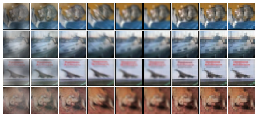Interpolations from the CVAE between fog, defocus blur, and pixelate corruptions.

Using adversarial examples from this perturbation set, we can train a CIFAR10 classifier that is robust to worst-case corruptions using adversarial training as described before. The following table summarizes the non-adversarial test set accuracy of a model trained with normal data augmentation (using all the common corruptions), CVAE data augmentation (using samples from the learned perturbation set) and adversarial training (using the learned perturbation set).

Method	Clean	Perturbed	Out of distribution
Data augmentation	90.6	87.7	85.0
CVAE data augmentation	94.5	90.5	89.6
Adversarial training	94.6	90.3	89.9

Performance of data augmentation and adversarial training on non-adversarial data

There are several interesting takeaways here. First, we find that both clean accuracy (measured on the original CIFAR10 dataset), perturbed accuracy (measured over the CIFAR10 images with common corruptions), and out of distribution accuracy (measured on 3 additional corruptions never seen before) all see improvements when training on the learned perturbation set over simply data augmenting with observed perturbations. This is in stark contrast to the usual trade off between standard and robust accuracy seen in the $\ell_p$ setting: rather than trading off standard performance for robust performance, adversarial training can actually improve both standard and robust performance! As a result, even if one does not care about worst-case robustness, learning a perturbation set from perturbed data can be a powerful tool for improving generalization on non-robust metrics over directly training on the perturbed data.

Method	Adversarial ($\epsilon = 2.7$)	Adversarial ($\epsilon = 3.9$)	Adversarial ($\epsilon = 10.2$)
Data augmentation	42.4	37.2	17.8
CVAE data augmentation	68.6	63.3	43.4
Adversarial training	72.1	66.1	55.6

Adversarial performance of data augmentation and adversarial training

This next table summarizes the adversarial performance, where adversarial robustness is with respect to the learned perturbation set. Less surprisingly, we observe that training on perturbed data with simple data augmentation does not confer worst-case robustness against the learned perturbation set. On the other hand, training with the learned perturbation set results in improved robustness to worst-case adversarial perturbations, with adversarial training (unsurprisingly) being the most robust. Some of these adversarial examples for the robust classifier are shown below:

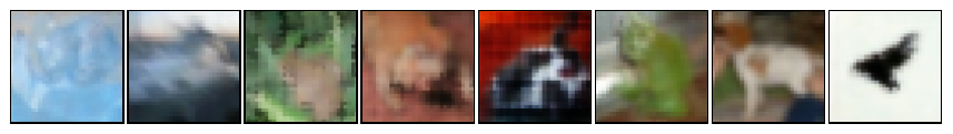Adversarial examples for a CIFAR10 classifier that is adversarially robust to common corruptions.

The main takeaway here is that by learning a model of perturbations that captures a diverse range of common corruptions, it is possible to both improve average robustness (both in and out of distribution) as well as adversarial robustenss on CIFAR10.

Robustness to changes in illumination

Another natural setting for studying perturbation sets is the Dataset of Multi-Illumination Images in the Wild. Here, data from 1000 different scenes found “in the wild” were photographed with 25 different lighting variations, from which a perturbation set can be learned to produce changes in lighting. For example, the following scene from a dining room was photographed with 25 different lighting variations as shown below:

images = multilum.query_images(['kingston_dining10'], mip=5)[0]
images = torch.from_numpy(images).contiguous().permute(0,3,1,2)

fig = plt.figure(figsize=(8,12))#, linewidth=4, edgecolor="#04253a")
grid = ImageGrid(fig, 111,  # similar to subplot(111)
                 nrows_ncols=(5, 5),  # creates 2x2 grid of axes
                 axes_pad=0.05,  # pad between axes in inch.
                 )
ims = make_grid(grid,images)

In this setting, we can learn a perturbation set in the same way as before, going through the same steps of (a) training a CVAE to reconstruct lighting perturbations, (b) calculating the radius for the latent space, and (c) using the generator to define a perturbation set. This perturbation set can then be used for downstream robustness to changes in lighting.

The downstream task we use for this dataset is image segmentation. Specifically, each scene is annotated with a material map which labels each pixel with a type of material (e.g. rug, wood, metal, etc.). The goal is to train an image segmentation model which learns to predict the material map of a given scene. An example of such a material map for the above dining room scene is shown below, which contains primarily foliage, wood, painted, and ceramic as the top four most occuring materials.

plt.imshow(materials)

We can then learn robust segmentation models using our learned perturbation set, e.g. by using adversarial training or randomized smoothing. We won’t go into too many details here, but we’ll highlight a randomized smoothing result: by training a typical UNet architecture to perform image segmentation, we can accurately predict 31% of the materials and certify 12% of these predictions to be robust to 50% of these lighting variations.

In this section, we only presented a couple experiments (adversarial training on CIFAR10 common corruptions, and randomized smoothing on the mutli-illumination dataset). However, there is no reason why we can’t use one of these robust training approaches on the other and vice versa, and a more comprehensive set of experiments can be found in our paper.

Summary

In this notebook, we tackled the problem of defining a perturbation set for real-world perturbations which cannot be easily described with a set of equations. We presented an approach based on generative modeling, using a latent space to capture variations in perturbations. We discussed how a generator can be learned with the CVAE framework, which we can show theoretically results in perturbation sets that satisfy the necessary subset and sufficient likelihood property, and can closely approximate a variety of perturbations in practice. These perturbation sets can then easily leverage existing methods in robust training (both empirical and provable), and can be used to learn robustness to image corruptions and lighting variations.

The main takeaway is that when we want to be robust to perturbations that are not as well-defined as the $\ell_p$ ball, when there is perturbed data available, it is possible to learn a perturbation set for training robust models to improve our machine learning models.

Learning perturbation sets for robust machine learning

Using generative modeling to capture real-world transformations from data for adversarial robustness

Table of contents